Supercharging DoorDash logistics through causal ML and joint optimization 

DoorDash’s delivery drivers — called Dashers — may be offered incentives such as peak pay (extra money) to improve supply during particularly busy times, in specific areas. Our supply system determines how many incentives are required based on predicted supply, demand, and incremental delivery quality improvements that likely would result from providing these incentives. 

Our assignment system optimizes, in real time, how to assign each delivery to a Dasher ¹. One of the key levers affecting these assignment results is batch rate — the percentage of deliveries assigned to the same Dasher in a single trip. In most supply conditions, increasing batch rate may save Dasher cost by minimizing duplicative travel, but may simultaneously degrade delivery duration, forcing consumers to endure longer waits because of these extra pickups and dropoffs. 

Problems

Originally, the supply system would determine a supply target for each geo or time unit based on cost and delivery quality trade-offs and utilization targets, defined as Dasher active time/online time, that describe how busy Dashers are. The system would also determine a total mobilization budget across all units based on overall costs and quality trade-offs. It then determined how much peak pay should be allocated to each geo or time unit to most effectively minimize undersupplied hours. More details about this previous system can be found in our engineering blog, Managing Supply and Demand Balance Through Machine Learning, that was published in 2021.

Hitting targets vs. improving supply

Our previous systems presented a conundrum: If we successfully optimized against targets, the systems would conclude — falsely — that there were no more benefits to improving supply. But better supply, of course, improves delivery quality and, eventually, long-term consumer volume. And because these supply targets are high-dimensional, static, and coarsely granular, it was difficult to guarantee that they were set optimally for every given unit. To top it all off, our estimates of how impactful peak pay could be on incremental hours and delivery quality were inherently biased because they were not derived through a causal machine learning (ML) framework.

Lack of system coordination 

Additional inefficiencies came from the relatively independent operations of the two systems. For example, on a Friday evening in downtown San Francisco, the assignment system might want to keep a high batch rate because supply was usually good and Dasher cost savings could outweigh the cost of increased delivery duration. But the supply system might set a low utilization target to boost supply because the delivery duration had not been ideal because of the high batch rate from the assignment system. The incremental costs of supply incentives, however, could be higher than the Dasher cost savings from the assignment system, while delivery quality remained suboptimal.

Solutions 

To resolve these problems, we removed the supply targets from both systems and instead directly optimized for consumer outcomes — in this case, delivery duration — by jointly making supply and assignment decisions based on causal estimates of their impact on delivery quality, Dasher cost, and mobilization cost. 

The primary challenges of this joint optimization system design are:

• Joint optimization complexity and scalability while managing nearly half a million geo and time units and two-dimensional decision variables 
• Estimating the joint impact of incentives and batch rate on delivery quality and cost
• Multi-stage decision making

Joint optimization 

The joint optimization system formulates the problem as a constrained integer programming model with two-dimensional decision variables: Peak pay amount and batch rate level. We discretized the batch rate decision variable (peak pay amount is naturally discretized) because its impact on Dasher cost and delivery duration is non-linear and it can make the problem tractable. This way, we can avoid solving a very complicated nonlinear mixed-integer programming model at such a large scale. 

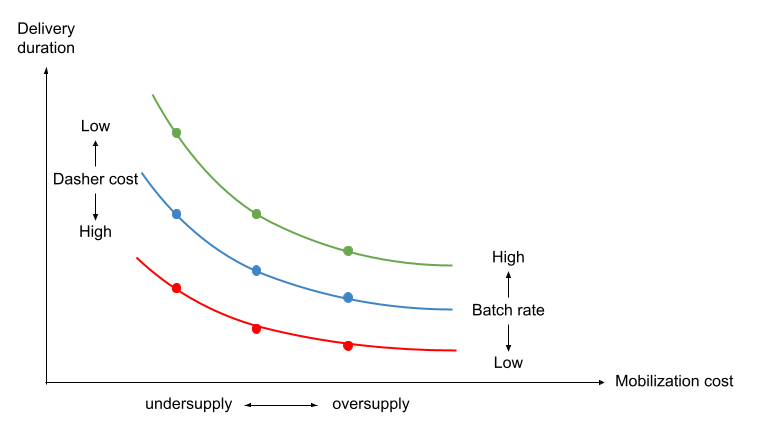
The key concept of this optimization problem is illustrated in Figure 1: 

• When we increase the mobilization cost, supply improvements and delivery duration decrease, but the relationship is non-linear and varies across different batch rate levels.
• When we decrease the batch rate, delivery duration can be reduced, but Dasher costs increase. The magnitude of these changes in delivery duration and Dasher cost also varies across different supply states. 

The objective function is to minimize the overall delivery duration subject to a total budget constraint on both mobilization and Dasher costs. The following is the mathematical formulation:

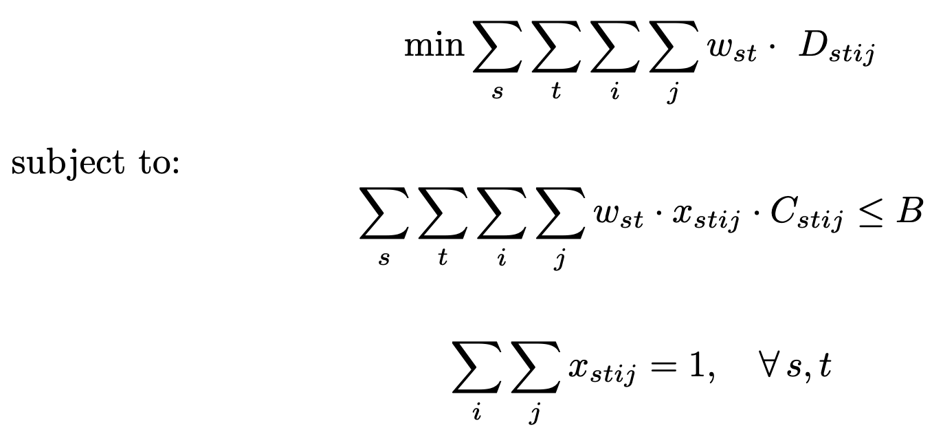
x_stij is the binary decision variable, 1 if (geo, time) unit (s, t) chooses peak pay level i and batch rate level j, 0 otherwise

w_st is the weight (volume) for (geo, time) unit (s, t)

D_stij is the average delivery duration for (geo, time) unit (s, t) with peak pay level i and batch rate level j; D_stij ~ f_st(x_stij)

C_stij is the total cost for (geo, time) unit (s, t) with peak pay level i and batch rate level j; C_stij ~ g_st(x_stij)

B is the total budget

The constraints require that our total cost cannot exceed the total budget and for each geo or  time unit, we can choose only one peak pay amount and batch rate level. 

We chose to minimize delivery duration in the objective function as a proxy for consumer long-term order volume, because it is one of the most important delivery quality factors within the logistics team's control. It is also highly correlated with other delivery quality metrics such as cancellation rate and late deliveries. We will share more details in a separate blog post about how we model the impact of delivery duration on long-term order volume.

Causal ML

The above optimization model’s performance is highly dependent on the accuracy of the input functions' estimation, as shown here:

• D_stij ~ f_st(x_stij)
• C_stij ~ g_st(x_stij)

Among the challenges of these function estimations are:

• Heterogeneity: These functions are quite heterogeneous across different geo and time units (s,t); in other words, they differ between the dinner rush and early morning hours or between urban and suburban settings, among other measures.
• Non-linearity: The impact of decision variables on delivery quality and cost is not linear, especially for batch rate.
• Interactions: Peak pay’s effect on quality can vary significantly at different batch rate levels.

What fell short

It might seem straightforward to fit an ML model based on observational data using delivery duration as the target variable, while treating peak pay, batch rate, and other variables as features. But this approach would lead to a highly biased causal effect estimation because the system only learns the correlation, not the causation. The observational data do not have a fully balanced feature distribution either of these two decision variables or other feature variables. If we had directly built this model, we would have estimated a false causal effect in which quality would worsen as peak pay rose because peak pay is usually added during undersupply conditions. 

Another option would be to train a double ML model using observational data. Unfortunately, this approach produces sub-optimal results and tends toward bias because delivery quality could be affected by many factors other than peak pay amount or batch rate. Additionally, double ML relies on two important assumptions to make sure the learned causal effects are unbiased: 1) There are no omitted confounding variables, and 2) no common effect variables are included. 

In the real world, there are so many systems and entities affecting each other that it’s rare to have a complete and clean causal directed acyclic graph that can guarantee the two assumptions are met. Such guarantees can usually only be ensured through using synthetic or randomized control trial (RCT) data.

Finding solutions

Our causal ML solutions followed these principles:

• Leveraging experimental RCT data as much as possible;
• Minimizing exploration costs when designing learning experiments; and
• Breaking down the causal chain from decision variable to final outcome variable — in this case delivery quality — by modeling the direct causal effect of decision variables and then relying on regular ML models to connect causal effects with final outcome variables.

Learning experiment design 

Ideally, we would run a switchback experiment with randomized peak pay and batch rate across all geo and time units, and use the results for causal ML learning. But that would be prohibitively expensive; we would have to randomly provide peak pay where it’s not needed — generating wasteful expenses — while also failing to provide peak pay when it’s actually needed, hurting delivery quality. Additionally, switchback experiments tend to have only moderate statistical power, which would mean running this randomized experiment at a large scale for multiple weeks. 

Instead, we decided to estimate the causal impact of peak pay on incremental supply hours first, then combine it with a downstream delivery duration prediction regular ML model. This takes the supply quality — for example, utilization — as one of the most important features, because this is the pathway through which peak pay impacts delivery duration. To do this, we designed a small exposure Dasher A/B learning experiment; because of its high power and minimum network effects at low exposure (more details in this blog post), we also ran multiple variants with both +$1 and -$1 to self-fund the experiment. 

Because batch rate is a continuous variable, it is not easy to set up learning experiments that explore all potential values. And because of the optimization challenges outlined above, we chose a few discrete batch rate values to run a multi-arm holdout switchback experiment that takes advantage of the fact that joint decision-making is granular for both geo and time. We also chose discrete values that would have a neutral average impact on quality. 

ML architecture

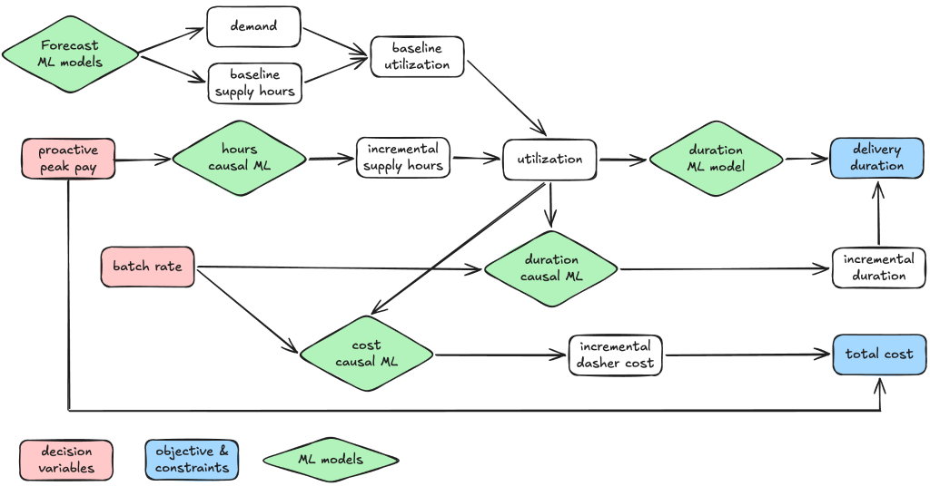
We have regular ML models that forecast demand and baseline supply hours for all geo and time units over a few days. We estimate the baseline supply state based on these forecasts, specifically baseline utilization. We then build a causal model to estimate the heterogeneous impacts of peak pay on incremental supply hours. By combining these two models, we derive the predicted utilization as a function of peak pay. Furthermore, we have a regular ML model that predicts delivery duration as a function of utilization and other features. Finally, by combining the duration prediction model and the utilization, we have the incremental delivery duration as a function of peak pay. 

From the batch rate learning experiment, we built two causal models that estimate the heterogeneous impacts of batch rate on incremental duration and Dasher cost, conditional on different utilization levels. Through combining the previous utilization model as a function of peak pay, we obtain the final delivery duration and total cost as a function of both peak pay and batch rate as shown in Figure 2.

Rather than modeling heterogeneous treatment effects (HTE) at the specific geo or time unit level for the batch rate causal models, utilization becomes the primary covariate variable. This improves model performance and generalization by capturing the key supply condition that drives how batch rate affects delivery duration and Dasher cost. The geo and time unit-level heterogeneous functions can therefore be rewritten as: 

• D_ij ~ f(x_ij | utilization, X)
• C_ij ~ g(x_ij | utilization, X)

In other words, we estimate the batch rate’s HTE on delivery duration and Dasher cost, conditional on utilization and other covariates X. From the batch rate learning experiment, we built two causal models conditioned on utilization — one for incremental delivery duration and one for Dasher cost. By combining these with the utilization model derived from the peak pay causal chain, we obtained the final delivery duration and total cost as a joint function of both peak pay and batch rate.  

As our base learner, we use R-learner with LightGBM across all three causal models. We chose R-learner because it tends to outperform S/T/X learners, supports both continuous and binary treatment variables, and works with both RCT and observational data, all of which make standardization straightforward and ease our ability to share modules across models. We chose LightGBM for its strong balance between model performance and complexity.

Validation 

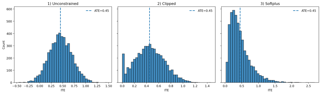
Causal model evaluation is difficult because we cannot directly observe the counterfactual or derivatives, instead observing only the outcome variable. Because we had generated RCT data, we used the cumulative gain and the Qini curve  area under uplift as the primary metrics for model selection based on out-of-sample data (hyperparameter tuning and feature/covariate selection). These are good at measuring the ranking performance of the predicted HTEs. However, because we aren’t only interested in ranking, but also in making direct decisions based on these causal predictions, the prediction value accuracy is important – weighted average HTE is equal to the average treatment effect (ATE). We need to ensure that the predicted HTE distribution makes real-world business sense. 

For example, incremental peak pay should have a non-negative impact on delivery quality regardless of geo or time unit. However, raw peak pay HTE predictions from R-learner tend to include a small fraction of negative values even though ATE is greater than zero. Because the outcome variable residual in the R-learner’s loss function is centered around zero, there is no guarantee that the predicted HTE will be either non-negative or non-positive. Even if we clip all negative peak pay effects to zero and rescale the distribution to make the new weighted average HTE match the ATE, that will mean that some units never receive any peak pay because predicted benefits to quality are zero, as described here: 

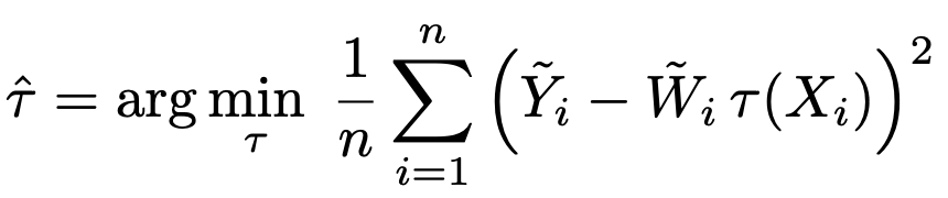
To solve this problem, instead of optimizing over 𝜏(𝑥) directly, we define 𝜏(𝑥) as a softplus function of another function g(x) (or other functions such as exponential or lognormal)

Then, we minimize the following loss function:

We can then obtain the final predicted HTE: 

Below are three example plots to illustrate the hypothetical predicted HTE distributions among: 1) raw predictions, 2) clipped and rescaled, and 3) constrained training

Multi-stage optimization

The above peak pay joint optimization allows us to proactively determine and publish peak pay, mobilizing Dashers more effectively to the correct geo and time units and allowing them to anticipate and plan their reactions. However, the more proactively we make decisions, the more likely we are to make mistakes based on lower forecast accuracy. 

As a result, we have a multi-stage joint optimization with both proactive and reactive systems. We will provide more details about the real-time joint optimization in a separate blog post. 

Conclusions and future directions 

We have validated through multiple A/B tests that the two-stage joint optimization system between supply and assignment not only significantly improves delivery quality but also reduces total cost. 

The following are some of the more helpful lessons we gleaned from this journey: 

• Look for systems that could benefit from joint optimization. Real-world systems are usually quite complex. In the early stages, complex problems can be broken down into independent subsystems to quickly resolve any issues. But when systems mature, it can be more beneficial to make joint decisions, especially for highly interdependent systems.
• Accurate forecast models and unbiased causal ML models are the key to successful optimization. 
• RCT data is the gold standard for building unbiased causal models. Try to design learning experiments that gather this data with enough power while still keeping exploration costs in check. 
• Prioritize different levels of causal modeling complexity. For example, at the initial proof of concept stage, we could use simple models or even just the ATE, but when there are enough signals and evidence, we can build more advanced models. 

Looking ahead, we’re excited about extending this framework to new frontiers, including:

• Real-time joint optimization between supply levers and demand levers
• Joint optimization between multiple supply levers beyond peak pay, such as base pay, acquisition cost, and demand shaping
• Considering both short-term and long-term effects of delivery quality on consumer engagement in the objective function.

Acknowledgements

Special thanks to Hao Quan, Yuxiang Yang, Yining Liu, Steffan Musoke, Abhijeet Bhorkar, Jeyda Kaynatma, and Alex Weinstein for their key contributions to this work. We also appreciate the discussions and valuable review comments from Fan Peng, Romil Bansal, Srinivasaraghavan Vedanarayanan, Eric Bencomo Dixon, Wilson Turner, Rachel Warner, Rob Hommel, Dan Madwed, Colin Schoppert, and Gayatri Iyengar.

Footnote

¹ While this blog post refers to the process of choosing a Dasher and sending an offer as an "assignment," this is a misnomer. Dashers are free to accept or decline any offer.