

Fraud doesn’t always kick the door down. More often, it starts quietly – hidden in the noise of millions of legitimate deliveries. A small spike in refund claims. A pattern in high-risk charges linked to a specific bank. A subtle shift in behavior that, left unchecked, can snowball into a costly, large-scale fraud trend.
DoorDash’s fraud team wanted to flip the script: Instead of reacting to a new fraud trend after it’s grown unchecked for weeks and finally starts to impact our top-line metrics, how could we spot the trend as early as possible — before significant damage is done?
This post shares how we built an anomaly detection platform to scan for emerging patterns across millions of user segments to surface the ones that matter before they spiral into major losses.
Because anomaly detection is a broad term with varying meanings even just within the fraud context, a brief introduction to terminology is in order. For the purposes of this blog, we’ll define two broad categories:
- Anomalous trend detection: Looking for anomalous behavior in a collection of users which may represent a new fraud or false-positive trend. Here, no particular datapoint may be anomalous, but a collection of data points together forms an anomaly. In this case, “anomaly” refers to an anomalous time-series, for example a growing fraud segment.
- Anomalous outlier detection: Looking for individual outliers — for instance, users or transactions — that are rare or deviate significantly from normal behavior. The individual datapoint is an anomaly; it may be part of a trend or it may be just a single anomaly.
This post focuses on the system we built at DoorDash to detect anomalous trends.
Below are some terms we’ll use throughout this post:
| Term | Definition | Examples |
| Metric | An early-warning metric that could indicate fraud or abuse | Number of credit and refund claims, dollar value of orders with a high chargeback model score |
| Dimension | An axis with which to slice the metrics | Customer_Country, Business_Name |
| Value | Value of a dimension | Customer_Country=’US’, Business_Name=’Retailer One’ |
| Segment | A single, double, or triple-product of dimension-value combinations. Segments are not mutually exclusive; many partially overlap with each other | {Customer_Country=’US’, Business_Name=’Retailer One’} |
| Anomaly | A time-series anomaly where a metric value is increasing within a given segment over a day-to-week timescale | Metric = # Credit & Refund claims, segment = {Customer_Country=’US’, Business_Name=’Retailer One’} |
| Cluster | A group of partially overlapping segments that share anomalies in the same metric | Metric = # Credit & Refund claims, {‘business_name’=’Retailer One’} &{‘country’=’US’, ‘business_name’=’Retailer One’} |
Developing the system
We started by talking to the frontline fraud teams responsible for tracking and fighting new fraud trends. We asked each team to give concrete historical examples of fraud trends that simmered for longer than ideal before being discovered and mitigated. These examples served as the positive test cases for our system.
We then asked the teams for their most useful early-warning indicator metrics, and collected a list of dimensions that they commonly use to slice and dice their data when they investigate new fraud trends.
This gave us a set of positive examples, metrics, and dimensions to use in our system. We then built and backtested the system, tuning the parameters as described in step 3 of Figure 1 below to maintain 100% recall on the test trends while minimizing the number of non-fraudulent anomalies per day. We observed that the system is fairly insensitive to the exact values of the tuning parameters; it is far more important to choose thoughtful metrics and dimensions to capture the fraud trends than it is to precisely tune the parameters.
System overview
The anomaly detection platform shown in Figure 1 runs as a daily job coordinated by Airflow to look for fraud trends that are growing on a day-to-week timescale. We currently have anomaly detection jobs running for both consumer fraud and Dasher fraud; we plan to expand to more applications over time.
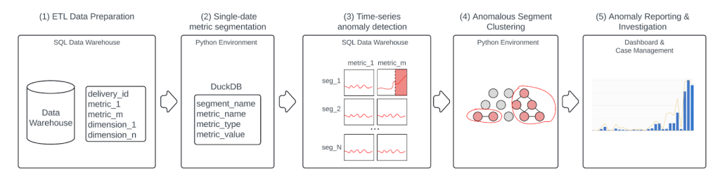
The system has five primary steps.
Step 1: Data warehouse extract-transform-load to prepare daily data
We chose a daily batch job for the initial implementation because most of the fraud trends that we historically missed developed over a few days to a few weeks. The Airflow directed acyclic graph prepares the dataset for each anomaly detection job containing the day’s data snapshot in wide-table format.
Step 2: Compute aggregates of metrics on multi-dimensional segments
We load the single date’s data into a Python environment via Spark and compute the aggregates of each metric across each segment. For each metric, we track both the absolute value of the metric — for example, $ Credit & Refund claims — and the relative, or normalized, value of the metric — for example, $ Credit & Refund claims/$ value of orders — to be used downstream in the anomaly detection step. We form segments from the single, double, and triple-product combinations of all our dimensions. This step boils down to computing aggregates of the metrics and then grouping them by several thousand different combinations.
| Dimensional product | # dimension products (excluding cardinality >107) | # segments |
| singlets | 30 | ~millions |
| doublets | ~hundreds | ~10s of millions |
| triplets | ~thousands | ~100s of millions |
We compute the metric aggregates using DuckDB, which is an in-memory Python database optimized for fast online analytical processing operations. We chose DuckDB because it is much faster — less than 10 minutes — than using Spark or Pandas-on-Spark and is more memory-efficient than Pandas. We exclude dimensional products with cardinality greater than 107 to reduce the total number of segments to a manageable size. The day’s metrics, aggregated across hundreds of millions of segments, are then stored in our data warehouse in sparse tall table format; in other words, we drop rows corresponding to segments with a metric value equal to zero to reduce storage space in both DuckDB and the downstream data warehouse.
Step 3: Time-series anomaly detection
The previous 28 days of data are stored in the data warehouse, so we now have several hundred million metric time series, each with a length of 28 days. We chose a simple moving-window z-score algorithm, which performed well in testing to detect all of our historical fraudulent trends. The first 21 days of each time series form the baseline, and the 28th day is the test day. We chose the seven-day gap between the baseline period and test day after noticing that many historical fraud trends had a noisy period when they first began to scale. By including this gap between the test and baseline, we get a better measurement of the true variance of the baseline prior to the trend scaling, which leads to fewer missed fraud trends.
We flag a given time series as anomalous if both of the following criteria are met:
- Statistical significance: 28th day relative metric is greater than X standard deviations above the mean of the 21-day baseline. We find 6 standard deviations works well empirically.
- Business significance: 28th day absolute metric exceeds the 21-day baseline by a dollar value and/or count that is business-significant for that metric; business significance thresholds are chosen in conjunction with our operations partners and can vary for different metrics.
Figure 2 below shows a visualization of a fictitious, but exemplary, anomaly.

Step 4: Hierarchical clustering on anomalous segments
A real fraud trend will often cause anomalous increases in a metric across many partially overlapping segments. For example, a spike in the number of credit and refund claims at Retailer One might cause anomalies in segments such as {‘business_name’=’Retailer One’}, {‘country’=’US’, ‘business_name’=’Retailer One’}, and {‘business_vertical’=’retail’, ‘business_name’=’Retailer One’}, as well as many other segments. To reduce the total number of anomalies that need to be investigated, we group partially overlapping anomalous segments using a custom hierarchical clustering algorithm.
The dimensional segments have a natural structure that can be represented by a three-layer graph with single-dimensional segments on the top layer, for example {‘business_name’=’Retailer One’}, dimensional-pairs on the middle layer, for example {‘business_name’=’Retailer One’, ‘country’=’US’}, and dimensional-triplets on the bottom layer, for example {‘business_name’=’Retailer One’, ‘country’=’US’, ‘checkout_platform’=’iOS’}. We further partition the graph by METRIC_NAME.
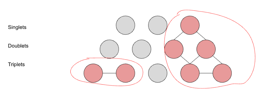
We then use a simple graph clustering algorithm to connect anomalies within the same metric_type:
- Connect all parent anomalies with their children anomalies
- {‘business_name’=’Retailer One’} is parent of {‘country’=’US’, ‘business_name’=’Retailer One’}
- {‘country’=’US’, ‘business_name’=’Retailer One’} is parent of {‘business_name’=’Retailer One’, ‘country’=’US’, ‘checkout_platform’=’iOS’}
- Connect sibling anomaly triplets if they share ⅔ of their keys and values
- {‘business_name’=’Retailer One’, ‘country’=’US’, ‘checkout_platform’=’iOS’} & {‘business_name’=’Retailer One’, ‘country’=’US’, ‘business_vertical’=’retail’} are connected as siblings.
We then run a graph partition algorithm to find the connected anomaly clusters. An example visualization showing how we cluster together parent and sibling anomalies is shown above in Figure 3. Downstream investigators review a cluster of segments together, starting by looking at a single segment that we choose as the representative of its cluster. We chose this representative segment using a fitness function:
fitness = abs_anom_amt * rel_amt / level1.2
Where abs_anom_amt is the value of the 28th-day metric minus the 21-day baseline; rel_amt is the relative (dollar or count-normalized) 28th day metric within the segment; and level=0 for dimensional singlets, 1 for pairs, and 2 for triplets. The idea behind this fitness function is to choose an anomalous segment that maximizes something analogous to an F-1 score (abs_anom_amount is analogous to recall, rel_amt is analogous to precision) but biases towards shallower or simpler segments through dividing by a weak function of the depth of dimensions.
In real-world operation, we typically see anomalies in several thousand segments each day. These typically are clustered into 20 to 60 anomalous clusters per day across various consumer and Dasher fraud areas, which is a volume that can be easily investigated by our operations team.
Step 5: Anomalous clusters are investigated in a workflow tool
Ultimately, the representative anomalous segments, along with all other segments in the cluster and example events such as deliveries and Dasher assignments, are accessible in a workflow tool for ops agent investigation. The agents review example deliveries or assignments within the representative anomalous segment, looking for common trends or patterns that may represent a new fraud trend. Sometimes the trends are determined to be non-fraudulent, for example a new promotion could lead to a spike in refunds, while at other times they are determined to be fraudulent. Trends that are deemed to be fraudulent are root-caused in partnership with engineering and product teams, so that the root cause can be addressed. Meanwhile, a separate containment team runs queries to identify and stop fraudsters matching the trend pattern until the product team can fix the root cause.
Impact
We now use the anomaly detection platform as our primary early-warning source for new fraudulent trends. More than 60% of all new fraud trends today are found through anomaly detection, and that number continues to grow as we add coverage to more fraud areas. Anomaly detection has brought the average time-to-detect new fraud trends down from more than 100 days to less than three days over the past year; this number will continue to drop as we cover more fraud areas. The platform saves us tens of millions of dollars per year by flagging small but growing fraud trends before they get out of control.
Future work
We plan to continue expanding the anomaly detection platform’s coverage to other fraud vectors and business applications within DoorDash. This technique applies well to growth, payments, and other business areas.
Currently, each daily batch of trends is investigated independently, often leading to similar clusters being re-investigated on multiple days. We plan to extend the clustering algorithm to run across recent days’ segments to reduce time wasted in redundant operator investigations.
We are looking into creating an AI agent to automate the review of anomalous trends and determine whether they are fraudulent or non-fraudulent. This is part of our broader team effort to use AI to automate manual investigations.
Conclusion
Fraud detection is most effective when it's proactive, not reactive. By building a scalable anomaly detection platform, we’ve enabled DoorDash to surface emerging fraud trends within days rather than weeks or months – before they cause significant damage. The system's flexibility, precision, and explainability empower our fraud teams to act swiftly and decisively. As we continue to expand coverage and layer in automation, this platform is becoming a cornerstone of our defense against fraud and a model for how data-driven engineering can create real business impact.