

We launched our new Consumer Packaged Goods (CPG) Interest Targeting initiative to let advertisers target consumers on new verticals (convenience stores, groceries, DashMart, etc.) based on their restaurant order history. Two key questions soon arose:
- Q1. Which consumer segments should I target?
- Q2. How does that selection change given different campaign objectives?
DoorDash is uniquely positioned to understand consumer preferences holistically, leveraging data from both sides of the business — restaurants and new verticals. But we needed to help advertisers translate those insights into actionable targeting tactics.
This was not an easy task. We had not previously explored how to map consumer behavior on the restaurant vertical into actionable new verticals insights, and we needed to figure out how to do it quickly enough to take advantage of advertiser excitement.
To answer both of our key questions, we designed a proprietary brand-dish affinity metric that quantifies, for any brand, how strongly each dish segment is correlated with conversions. With a per-segment strength score in hand, advertisers can use interest targeting as a performance lever to spend budgets more efficiently on high-affinity segments, or reach new audiences with tailored creatives for innovation products. We expose these scores in a self-serve report so advertisers can explore and experiment.
What is brand affinity?
We define brand affinity to a dish segment as how much more likely customers in the segment are to convert on the brand's ad than customers outside it. Higher affinity means stronger lift from targeting that segment.
To illustrate this, we can look at a hypothetical soda brand’s affinities across various segments, as shown in Table 1.
| Dish Segment | Conversion Rate In Segment | Conversion Rate Not in Segment | Brand Affinity |
| Tacos | 1.92% | 1.62% | 0.17 |
| Burgers | 2.35% | 2.04% | 0.14 |
| Pasta | 2.10% | 1.88% | 0.11 |
| Fries | 2.42% | 2.21% | 0.09 |
| Salads | 1.78% | 1.73% | 0.03 |
| Coffee | 1.65% | 1.70% | -0.03 |
| Sushi | 1.58% | 1.71% | -0.08 |
| Smoothies | 1.45% | 1.65% | -0.13 |
The affinity score helps assess a segment’s unique value for targeting. In this example, customers who frequently purchase tacos have the highest affinity (0.17) for the brand's ad, meaning they are disproportionately more likely to convert; the tacos segment, therefore, is more efficient and profitable. Conversely, the smoothies segment has the lowest affinity (-0.13), suggesting this group is less likely to convert than those outside of it. That signals headroom: A chance to connect with this segment through tailored campaigns and moments, ultimately moving smoothies up the ranks if the brand is willing to invest. Finally, the salads segment sits near zero affinity (0.03), which means it is a neutral choice that can extend reach without meaningfully helping or hurting performance.
Less effective alternatives
Go simpler. A naive alternative is to rank segments by raw conversion rate (CVR) as shown in Table 1, column 2. But this breaks down quickly; a broadly popular brand will convert well in almost every segment, but that does not mean any one segment has a special relationship with it. When in-segment and out-of-segment rates are both high, the contrast we care about disappears. In the example above, the category ”fries” has the highest raw in-segment CVR but only the fourth-highest affinity, because conversion is also high outside the segment. Affinity is designed to capture contrast, not level.
Go fancier. At the other extreme, we could train a machine-learning model to predict brand conversion at the impression or consumer level, using hundreds of features and brand-dish interactions. That would likely capture rich signals, but it would demand far more infrastructure, calibration, and ongoing maintenance than a transparent score, while denying advertisers the ability to reason about why a segment is strong.
Our affinity score sits in the sweet spot: Simple enough to communicate, principled enough to extend.
Computing the affinity score
The affinity score is calculated using this log-odds ratio:
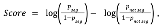
where pseg represents the probability of conversion inside the segment and pnot seg is the probability outside of it.
This compares how likely a customer in the segment is to convert relative to someone outside the segment, expressed on the log-odds scale. Raw probability differences capture absolute lift, but affinity is fundamentally about relative changes in conversion propensity. A segment that doubles conversion from 0.2% to 0.4% signals a much stronger behavioral effect than a segment that moves conversion from 4.2% to 4.4%, even though both represent the same absolute lift. Odds ratios capture this notion of relative change naturally. Taking the logarithm then maps multiplicative effects onto an additive scale: a 2× increase and a 2× decrease correspond to equal-magnitude scores with opposite signs. The result is a comparable and interpretable scale that can be compared across brands with very different baseline conversion rates.
In short, the affinity score highlights where a segment makes a brand's customers meaningfully more or less likely to convert, expressed in a stable and comparable way across segments.
Statistical interpretation
The log-odds calculation above already provides an interpretable ranking of segments for a brand. In this section, we show a principled approach that both recovers that definition and quantifies uncertainty. Quantifying uncertainty is fundamental: A high affinity based on millions of impressions should inspire more confidence than the same score based on a small sample. This calls for testing whether the score is statistically distinguishable from zero, which arises naturally once we express the metric as a statistical model.
The following is a logistic-regression view of the same metric. Let Yc ϵ{0,1} indicate whether the consumer c converts, and Sc ϵ{0,1} whether they belong to the segment S. The simplest model is:
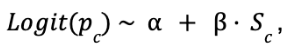
where
- Pc = Pr[Yc=1] is the consumer's conversion probability,
- 𝛂 is the baseline log-odds of conversion to the brand, and
- 𝛃 is the incremental log-odds associated with belonging to the segment.
That 𝛃 is our affinity score. In the binary case, the fitted coefficient is the difference in log-odds between consumers inside and outside the segment. The metric is not an ad hoc heuristic; it arises from a canonical statistical model.
When we look at uncertainty at scale, fitting the regression gives us a standard error on 𝛃 for free. From there, we can build confidence intervals and test whether an affinity is statistically distinguishable from zero. That matters when comparing segments with very different sample sizes: A score of 0.15 estimated on millions of impressions carries a significantly different weight than the same score on a few thousand.
This gives us a principled way to answer questions such as:
- Is this segment truly over-indexing, or could the observed lift be noise?
- Which affinities are strong enough to surface confidently in an advertiser-facing report?
- Which affinities represent genuine brand-specific behavior rather than patterns explained by overall conversion rates or segment prevalence?
We have a key advantage here: The framing for one model scales to all segments. Instead of fitting a separate comparison for each dish, we write a single consumer-level model as shown here with one indicator per segment:
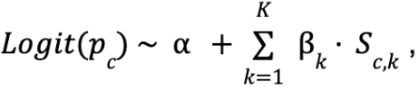
where Sc,k indicates whether the consumer c belongs to the segment k. Each coefficient 𝛃k is that segment's affinity, all estimated jointly within the same statistical framework. Operationally, this is much cleaner: One fit produces a full vector of affinities, standard errors, and confidence intervals, rather than treating each segment as a separate, standalone calculation.
Generalizations
Conversion rate is a useful and intuitive default on which to get started. We can keep that same broader thought process as we expand to meet other advertiser goals: Compare outcomes inside and outside each segment, rank segments by how much they over-index, and use that ranking to guide targeting. What changes is the outcome being modeled. Moving from CVR to incremental sales, units, or profit may require a different statistical formulation, but not a different decision framework.
Another immediate extension is adjusted affinity. Adding covariates to the same regression lets us separate segment-specific signals from broader differences in customer composition, such as heavy vs. light users, new vs. existing-to-brand, geography, or daypart. An unadjusted affinity can overstate a segment where consumers are simply more active on DoorDash overall; an adjusted version isolates the portion of lift that is genuinely about the segment.
The more ambitious direction is to let data, rather than advertisers, pick the target segments. Today, an advertiser browses the affinity ranking and chooses the top few by hand. This is a workable approach, but it leaves the final call to intuition and treats every segment as a separate question. A more scalable path is to evaluate all segments for a brand jointly against a chosen objective — say sales, new-to-brand rate, or return on ad spend. We could then use regularized regression or related variable-selection methods to surface only the segments that carry real, non-redundant signals. The interesting questions multiply from there, but the general direction moves toward optimization-based, data-informed targeting.
Key takeaways
In building brand-dish affinity, we set out initially to answer two core questions for advertisers seeking to deploy interest targeting. We were able to use affinity rankings to tell them immediately which consumer segments have the strongest relationship with the brand and are therefore the best candidates to target. That led naturally to an answer for the second question about how the selection should change given varying campaign objectives: Keep the same ranking logic, but swap in the advertiser's objective. The current metric then becomes both a practical solution to the first problem and a principled foundation for the second. More broadly, it represents a first step toward fully data-driven audience optimization.
Brand affinity allows advertisers to better understand their current consumer reach and identify groups with whom they can improve their connection. By providing them with that data in an easily digestible score, advertisers can maximize their efficiency and plan future campaigns to address opportunities revealed through brand affinity.
